Note
Click here to download the full example code
PPG Pre-processing and SQI Calculations using Pandas
Trimming, Filtering, Segmentation and SQI Calculations utilising Pandas
9 10 11 12 | # Code Adapted from:
# https://meta00.github.io/vital_sqi/_examples/others/plot_pipeline_02.html
# AND
# https://meta00.github.io/vital_sqi/_examples/others/plot_read_signal.html#sphx-glr-examples-others-plot-read-signal-py
|
16 17 18 19 20 21 | '''
This file will be used in calculating the SQIs for each patient (and discarding parts of the signal soon).
A loop will be implemented in future iterations for the different patiend files. In general, the file is built
parametrically so that the procedure can be automated.
'''
|
Out:
'\nThis file will be used in calculating the SQIs for each patient (and discarding parts of the signal soon).\nA loop will be implemented in future iterations for the different patiend files. In general, the file is built\nparametrically so that the procedure can be automated.\n\n'
Importing Libraries
25 26 27 28 29 30 31 32 33 34 35 36 37 38 39 40 41 42 | # Generic
import os
import numpy as np
import pandas as pd
import matplotlib.pyplot as plt
from scipy import signal
from datetime import datetime
# Scipy
from scipy.stats import skew, kurtosis, entropy
# vitalSQI
from vital_sqi.data.signal_io import PPG_reader
import vital_sqi.highlevel_functions.highlevel as sqi_hl
import vital_sqi.data.segment_split as sqi_sg
from vital_sqi.common.rpeak_detection import PeakDetector
from vital_sqi.preprocess.band_filter import BandpassFilter
import vital_sqi.sqi as sq
|
Loading data
48 49 50 51 52 53 54 55 56 57 58 59 60 61 62 63 64 65 66 67 68 69 70 71 72 73 74 75 76 77 78 79 80 81 82 83 84 85 86 87 | # Filepath definition
filepath = r'..\..\..\..\OUCRU\01NVa_Dengue\Adults\01NVa-003-2001\PPG'
filename = r'01NVa-003-2001 Smartcare.csv'
filename_Clinical = r'..\..\..\..\OUCRU\Clinical\v0.0.10\01nva_data_stacked_corrected.csv'
#defining constants
trim_amount = 300
hp_filt_params = (1, 1) #(Hz, order)
lp_filt_params = (20, 4) #(Hz, order)
filter_type = 'butter'
segment_length = 30
sampling_rate = 100
#reading Clinical Data
Clinical = pd.read_csv(filename_Clinical)
#readind PPG data
data = pd.read_csv(os.path.join(filepath, filename))
# data = PPG_reader(os.path.join(filepath, filename),
# signal_idx=["PLETH", "IR_ADC"],
# timestamp_idx=["TIMESTAMP_MS"],
# info_idx=["SPO2_PCT","PULSE_BPM","PERFUSION_INDEX"], sampling_rate=sampling_rate)
print(data)
print(data.PLETH)
print(data.IR_ADC)
print(data.TIMESTAMP_MS)
print(data.SPO2_PCT)
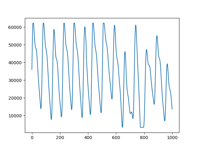
signals = data[["PLETH", "IR_ADC"]]
plot_range = np.arange(0,1000,1)
fig, ax = plt.subplots()
ax.plot(plot_range, signals.iloc[0:1000, 0])
|
Out:
         TIMESTAMP_MS  COUNTER  DEVICE_ID  PULSE_BPM  SPO2_PCT  SPO2_STATUS  PLETH  BATTERY_PCT  RED_ADC  IR_ADC  PERFUSION_INDEX
0                   0        9          1         82      97.1            0  36033        100.0   144180  216524              4.4
1                  10       10          1         82      97.1            0  40919        100.0   144160  216470              4.4
2                  20       11          1         82      97.1            0  45715        100.0   144158  216415              4.4
3                  30       12          1         82      97.1            0  50227        100.0   144148  216364              4.4
4                  40       13          1         82      97.1            0  54362        100.0   144132  216379              4.4
...               ...      ...        ...        ...       ...          ...    ...          ...      ...     ...              ...
5626372      56269900  5626999          1         78      91.4            0  31408          5.7   292213  183755              5.6
5626373      56269910  5627000          1         78      91.4            0  31318          5.7   292557  184002              5.6
5626374      56269920  5627001          1         78      91.4            0  31117          5.7   292840  184296              5.6
5626375      56269930  5627002          1         78      91.4            0  30761          5.7   293161  184554              5.6
5626376      56269940  5627003          1         78      91.4            0  30261          5.7   293522  184828              5.6

[5626377 rows x 11 columns]
0          36033
1          40919
2          45715
3          50227
4          54362
           ...
5626372    31408
5626373    31318
5626374    31117
5626375    30761
5626376    30261
Name: PLETH, Length: 5626377, dtype: int64
0          216524
1          216470
2          216415
3          216364
4          216379
            ...
5626372    183755
5626373    184002
5626374    184296
5626375    184554
5626376    184828
Name: IR_ADC, Length: 5626377, dtype: int64
0                 0
1                10
2                20
3                30
4                40
             ...
5626372    56269900
5626373    56269910
5626374    56269920
5626375    56269930
5626376    56269940
Name: TIMESTAMP_MS, Length: 5626377, dtype: int64
0          97.1
1          97.1
2          97.1
3          97.1
4          97.1
           ...
5626372    91.4
5626373    91.4
5626374    91.4
5626375    91.4
5626376    91.4
Name: SPO2_PCT, Length: 5626377, dtype: float64

[<matplotlib.lines.Line2D object at 0x000001C5BCEA4B50>]
fetching ppg_start time
91 92 93 | def find_event_ppg_time(Clinical,Patient):
row = Clinical[(Clinical.study_no == Patient) & (Clinical.column == 'event_ppg') & (Clinical.result == 'True')]
return row['date'].values
|
Setting the indexes for the raw data - adopted from examples
97 98 99 100 101 102 103 104 105 106 107 108 109 110 111 112 113 114 115 116 117 118 119 120 121 122 123 124 125 126 127 | pd.Timedelta.__str__ = lambda x: x._repr_base('all')
#Transposing data.signals to set into columns
#signals = pd.DataFrame(data.signals.T)
# Include column with index
signals = signals.reset_index()
signals['timedelta'] = pd.to_timedelta(data.TIMESTAMP_MS, unit='ms')
PPG_start_date = find_event_ppg_time(Clinical, filename.split()[0][-8:])
PPG_start_date = datetime.strptime(PPG_start_date[0], '%Y-%m-%d %H:%M:%S')
signals['PPG_Datetime'] = pd.to_datetime(PPG_start_date)
signals['PPG_Datetime']+= pd.to_timedelta(signals.timedelta)
# Set the timedelta index (keep numeric index too)
signals = signals.set_index('timedelta')
# Rename column to avoid confusion
signals = signals.rename(columns={'index': 'idx'})
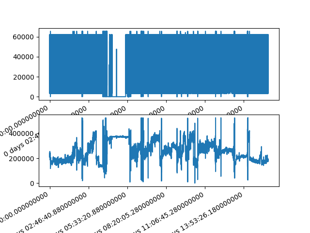
print("Raw Signals:")
print(signals)
#Plotting
fig, axes = plt.subplots(nrows=2, ncols=1)
axes = axes.flatten()
signals.iloc[:,1].plot(ax=axes[0])
signals.iloc[:,2].plot(ax=axes[1])
|
Out:
Raw Signals:
                            idx  PLETH  IR_ADC            PPG_Datetime
timedelta
0 days 00:00:00               0  36033  216524 2020-06-04 09:05:00.000
0 days 00:00:00.010000        1  40919  216470 2020-06-04 09:05:00.010
0 days 00:00:00.020000        2  45715  216415 2020-06-04 09:05:00.020
0 days 00:00:00.030000        3  50227  216364 2020-06-04 09:05:00.030
0 days 00:00:00.040000        4  54362  216379 2020-06-04 09:05:00.040
...                         ...    ...     ...                     ...
0 days 15:37:49.900000  5626372  31408  183755 2020-06-05 00:42:49.900
0 days 15:37:49.910000  5626373  31318  184002 2020-06-05 00:42:49.910
0 days 15:37:49.920000  5626374  31117  184296 2020-06-05 00:42:49.920
0 days 15:37:49.930000  5626375  30761  184554 2020-06-05 00:42:49.930
0 days 15:37:49.940000  5626376  30261  184828 2020-06-05 00:42:49.940

[5626377 rows x 4 columns]

<AxesSubplot:xlabel='timedelta'>
Trimming the first and last 5 minutes
132 133 134 135 136 137 138 139 140 141 142 | #Defining the 5 minute offset
offset = pd.Timedelta(minutes=5)
#Indexes - adopted from example
idxs = (signals.index > offset) & \
(signals.index < signals.index[-1] - offset)
#Trimming
signals = signals[idxs]
print(signals)
|
Out:
                            idx  PLETH  IR_ADC            PPG_Datetime
timedelta
0 days 00:05:00.010000    29913  21755  188656 2020-06-04 09:10:00.010
0 days 00:05:00.020000    29914  23262  187701 2020-06-04 09:10:00.020
0 days 00:05:00.030000    29915  25285  186998 2020-06-04 09:10:00.030
0 days 00:05:00.040000    29916  27839  186472 2020-06-04 09:10:00.040
0 days 00:05:00.050000    29917  30888  186113 2020-06-04 09:10:00.050
...                         ...    ...     ...                     ...
0 days 15:32:49.890000  5596371  15083  186186 2020-06-05 00:37:49.890
0 days 15:32:49.900000  5596372  13923  186422 2020-06-05 00:37:49.900
0 days 15:32:49.910000  5596373  12818  186662 2020-06-05 00:37:49.910
0 days 15:32:49.920000  5596374  11769  186807 2020-06-05 00:37:49.920
0 days 15:32:49.930000  5596375  10763  186899 2020-06-05 00:37:49.930

[5566463 rows x 4 columns]
147 148 149 | # RESAMPLE??
# MISSING DATA INPUT??
# TAPPERING??
|
Band-pass filtering
154 155 156 157 158 159 160 161 162 163 164 165 166 167 168 169 170 171 172 173 174 175 176 177 178 179 | '''
Band-pass filtering can be adjusted, maybe use a lower low-pass
cutoff frequency @15-17Hz
'''
#Band pass filtering function
def bpf(signal):
hp_filt_params = (1, 1) #(Cutoff Hz, order)
lp_filt_params = (20, 4) #( Cutoff Hz, order)
sampling_rate = 100
filter = BandpassFilter(band_type='butter', fs=sampling_rate)
filtered_signal = filter.signal_highpass_filter(signal, cutoff=hp_filt_params[0], order=hp_filt_params[1])
filtered_signal = filter.signal_lowpass_filter(filtered_signal, cutoff=lp_filt_params[0], order=lp_filt_params[1])
return filtered_signal
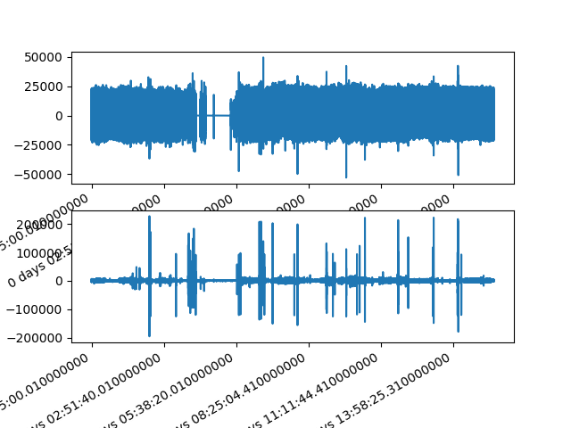
#Band-pass filtered signals
signals['PLETH_bpf'] = bpf(signals.iloc[:,1])
signals['IR_ADC_bpf'] = bpf(signals.iloc[:,2])
print('Raw and Filtered Signals:')
print(signals)
fig, axes = plt.subplots(nrows=2, ncols=1)
axes = axes.flatten()
signals['PLETH_bpf'].plot(ax=axes[0])
signals['IR_ADC_bpf'].plot(ax=axes[1])
|
Out:
Raw and Filtered Signals:
                            idx  PLETH  IR_ADC            PPG_Datetime    PLETH_bpf   IR_ADC_bpf
timedelta
0 days 00:05:00.010000    29913  21755  188656 2020-06-04 09:10:00.010  -214.886697   -32.494545
0 days 00:05:00.020000    29914  23262  187701 2020-06-04 09:10:00.020 -1224.999347  -226.831554
0 days 00:05:00.030000    29915  25285  186998 2020-06-04 09:10:00.030 -3047.445501  -734.950280
0 days 00:05:00.040000    29916  27839  186472 2020-06-04 09:10:00.040 -4351.721824 -1499.309485
0 days 00:05:00.050000    29917  30888  186113 2020-06-04 09:10:00.050 -3863.561589 -2230.015638
...                         ...    ...     ...                     ...          ...          ...
0 days 15:32:49.890000  5596371  15083  186186 2020-06-05 00:37:49.890   942.030869    45.325519
0 days 15:32:49.900000  5596372  13923  186422 2020-06-05 00:37:49.900   708.195771    93.296871
0 days 15:32:49.910000  5596373  12818  186662 2020-06-05 00:37:49.910   542.754581   127.077955
0 days 15:32:49.920000  5596374  11769  186807 2020-06-05 00:37:49.920   442.131641   151.598399
0 days 15:32:49.930000  5596375  10763  186899 2020-06-05 00:37:49.930   402.889073   159.679506

[5566463 rows x 6 columns]

<AxesSubplot:xlabel='timedelta'>
SQI Functions Definition and Peak Detection
185 186 187 188 189 190 191 192 193 194 195 196 197 198 199 200 201 202 203 204 205 206 207 208 209 210 211 212 213 214 215 216 217 218 219 220 221 222 223 224 225 226 227 228 229 230 231 232 233 234 235 236 237 238 | def PeakDetection(x):
detector = PeakDetector()
peaks, troughs = detector.ppg_detector(x, 7) #6 and 7 work the best
return peaks, troughs
#Defining SQI Functions
def snr(x):
#Signal to noise ratio
#needs raw signal
return np.mean(sq.standard_sqi.signal_to_noise_sqi(x))
def zcr(x):
#Zero Crossing Rate
#Needs filtered signal
return 0.5 * np.mean(np.abs(np.diff(np.sign(x))))
def mcr(x):
#Mean Crossing Rate
#needs raw signal
return zcr(x - np.mean(x))
def perfusion(x,y):
return (np.max(y) - np.min(y)) / np.abs(np.mean(x)) * 100
def correlogram(x):
#Correlogram
#Needs filtered signal
return sq.rpeaks_sqi.correlogram_sqi(x)
#Calculating peaks and troughs using peakdetector function for both filtered signals
peak_list_0, trough_list_0 = PeakDetection(signals['PLETH_bpf'])
peak_list_1, trough_list_1 = PeakDetection(signals['IR_ADC_bpf'])
'''
MSW values that are being calculated are too small, maybe peakdetectors need
to be revisited?
'''
def msq(x,peaks):
#Dynamic Time Warping
#Requires Filtered Signal and peaks
# Return
return sq.standard_sqi.msq_sqi(x, peaks_1=peaks, peak_detect2=6)
'''
Below function is outputting an error, needs revisiting
'''
# def dtw(x,troughs):
# #Dynamic Time Warping
# #Requires Filtered Signal and troughs and template selection 0-3 (0-2 for PPG)
# # Per beat
# dtw_list = sq.standard_sqi.per_beat_sqi(sqi_func=sq.dtw_sqi, troughs=troughs, signal=x, taper=True, template_type=1)
# # Return mean and standard deviation
# return [np.mean(dtw_list), np.std(dtw_list)]
|
Out:
'\nBelow function is outputting an error, needs revisiting\n'
Function Computing SQIs
243 244 245 246 247 248 249 250 251 252 253 254 255 256 257 258 259 260 261 262 263 264 265 266 267 268 269 | def sqi_all(x,raw,filtered,peaks,troughs):
#Computing all SQIs using the functions above
# Information
dinfo = {
'PPG_w_s': x.PPG_Datetime.iloc[0],
'PPG_w_f': x.PPG_Datetime.iloc[-1],
'first': x.idx.iloc[0],
'last': x.idx.iloc[-1],
'skew': skew(x[raw]),
'entropy': entropy(x[raw]),
'kurtosis': kurtosis(x[raw]),
'snr': snr(x[raw]),
'mcr': mcr(x[raw]),
'zcr': zcr(x[filtered]),
'msq': msq(x[filtered],peaks),
'perfusion': perfusion(x[raw], x[filtered]),
'correlogram': correlogram(x[filtered]),
#'dtw': dtw(x[filtered],troughs)
}
'''
When using dtw an empty signal error is presented that
needs fixing, not sure why it does that
'''
# Return
return pd.Series(dinfo)
|
Calculating SQIs for both signals 0 = Pleth and 1 = IR_ADC
274 275 276 277 278 279 280 281 282 283 284 285 286 287 288 289 | sqis_0 = signals.groupby(pd.Grouper(freq='30s')).apply(lambda x: sqi_all(x, 'PLETH','PLETH_bpf', peak_list_0, trough_list_0))
sqis_1 = signals.groupby(pd.Grouper(freq='30s')).apply(lambda x: sqi_all(x, 'IR_ADC','IR_ADC_bpf', peak_list_1, trough_list_1))
#Displaying the SQIs per signal
print("SQIs Signal 0 (Pleth):")
sqis_0
print(sqis_0)
print("SQIs Signal 1 (IR_ADC):")
sqis_1
print(sqis_1)
sqis_1 = sqis_1.drop(['first','last', 'PPG_w_s', 'PPG_w_f'], axis = 1)
# Add window id to identify point of shock more easily
sqis_1['w'] = np.arange(sqis_1.shape[0])
|
Out:
d:\files\desktop\dissertation icl\env\lib\site-packages\statsmodels\tsa\stattools.py:667: FutureWarning: fft=True will become the default after the release of the 0.12 release of statsmodels. To suppress this warning, explicitly set fft=False.
  warnings.warn(
SQIs Signal 0 (Pleth):
                                       PPG_w_s                 PPG_w_f    first  ...       msq   perfusion                                        correlogram
timedelta                                                                        ...
0 days 00:05:00.010000 2020-06-04 09:10:00.010 2020-06-04 09:10:30.000    29913  ...  0.000438  131.768567  [75, 150, 225, 0.9247323846304137, 0.836659565...
0 days 00:05:30.010000 2020-06-04 09:10:30.010 2020-06-04 09:11:00.000    32913  ...  0.000037  129.721286  [74, 148, 222, 0.9374430072923502, 0.866928327...
0 days 00:06:00.010000 2020-06-04 09:11:00.010 2020-06-04 09:11:30.000    35913  ...  0.000000  135.690506  [75, 150, 225, 0.9244827555340438, 0.814277364...
0 days 00:06:30.010000 2020-06-04 09:11:30.010 2020-06-04 09:12:00.000    38913  ...  0.000007  136.156223  [75, 150, 225, 0.9386014677175014, 0.862369440...
0 days 00:07:00.010000 2020-06-04 09:12:00.010 2020-06-04 09:12:30.000    41913  ...  0.000000  139.046179  [74, 149, 224, 0.9313743004418997, 0.824739899...
...                                        ...                     ...      ...  ...       ...         ...                                                ...
0 days 15:30:30.010000 2020-06-05 00:35:30.010 2020-06-05 00:36:00.000  5582383  ...  0.000000  148.508917  [37, 74, 110, -0.3912006306694429, 0.952924647...
0 days 15:31:00.010000 2020-06-05 00:36:00.010 2020-06-05 00:36:30.000  5585383  ...  0.000022  138.961305  [37, 75, 112, -0.38664616039771205, 0.95837555...
0 days 15:31:30.010000 2020-06-05 00:36:30.010 2020-06-05 00:37:00.000  5588383  ...  0.000015  125.616461  [77, 153, 230, 0.9462808953640326, 0.887181765...
0 days 15:32:00.010000 2020-06-05 00:37:00.010 2020-06-05 00:37:30.000  5591383  ...  0.000015  135.269077  [36, 74, 110, -0.37596691904957935, 0.93875374...
0 days 15:32:30.010000 2020-06-05 00:37:30.010 2020-06-05 00:37:49.930  5594383  ...  0.000022  134.870996  [37, 75, 112, -0.36633265827700123, 0.94094953...

[1856 rows x 13 columns]
SQIs Signal 1 (IR_ADC):
                                       PPG_w_s                 PPG_w_f    first  ...       msq  perfusion                                        correlogram
timedelta                                                                        ...
0 days 00:05:00.010000 2020-06-04 09:10:00.010 2020-06-04 09:10:30.000    29913  ...  0.000319   6.653209  [75, 150, 226, 0.9132608947040779, 0.799647163...
0 days 00:05:30.010000 2020-06-04 09:10:30.010 2020-06-04 09:11:00.000    32913  ...  0.000013   5.641682  [74, 148, 222, 0.9164960001123641, 0.827303342...
0 days 00:06:00.010000 2020-06-04 09:11:00.010 2020-06-04 09:11:30.000    35913  ...  0.000008   6.088179  [75, 150, 225, 0.9097936306566979, 0.779681593...
0 days 00:06:30.010000 2020-06-04 09:11:30.010 2020-06-04 09:12:00.000    38913  ...  0.000013   4.644686  [75, 149, 224, 0.9128541336509863, 0.807913379...
0 days 00:07:00.010000 2020-06-04 09:12:00.010 2020-06-04 09:12:30.000    41913  ...  0.000000   4.241945  [74, 149, 223, 0.9123059092032415, 0.791340070...
...                                        ...                     ...      ...  ...       ...        ...                                                ...
0 days 15:30:30.010000 2020-06-05 00:35:30.010 2020-06-05 00:36:00.000  5582383  ...  0.000013   4.946963  [34, 74, 107, -0.38922458037787383, 0.95155578...
0 days 15:31:00.010000 2020-06-05 00:36:00.010 2020-06-05 00:36:30.000  5585383  ...  0.000000   4.268080  [75, 150, 226, 0.964216933015672, 0.9155762504...
0 days 15:31:30.010000 2020-06-05 00:36:30.010 2020-06-05 00:37:00.000  5588383  ...  0.000013   4.733346  [77, 153, 230, 0.9423859574341878, 0.877431048...
0 days 15:32:00.010000 2020-06-05 00:37:00.010 2020-06-05 00:37:30.000  5591383  ...  0.000008   4.645047  [74, 103, 148, 0.9269084193473138, -0.35288054...
0 days 15:32:30.010000 2020-06-05 00:37:30.010 2020-06-05 00:37:49.930  5594383  ...  0.000008   4.352384  [75, 150, 226, 0.9326593121930683, 0.859995140...

[1856 rows x 13 columns]
Final Formatting into a single DataFrame and Saving into a .csv file
295 296 297 298 299 300 301 302 303 | #Merging SQIs of different signals from the same record (Pleth and IR_ADC)
Signal_SQIs = sqis_0.merge(sqis_1, on='timedelta', suffixes=('_0', '_1'))
#Automatically fetching the study_no from the filename and including it in the DataFrame
Signal_SQIs['study_no'] = filename.split()[0][-8:]
print(Signal_SQIs)
# Saving the SQIs to a CSV file
Signal_SQIs.to_csv(r'..\..\..\..\OUCRU\Outputs\SQI.csv')
|
Out:
                                       PPG_w_s                 PPG_w_f    first  ...                                      correlogram_1     w  study_no
timedelta                                                                        ...
0 days 00:05:00.010000 2020-06-04 09:10:00.010 2020-06-04 09:10:30.000    29913  ...  [75, 150, 226, 0.9132608947040779, 0.799647163...     0  003-2001
0 days 00:05:30.010000 2020-06-04 09:10:30.010 2020-06-04 09:11:00.000    32913  ...  [74, 148, 222, 0.9164960001123641, 0.827303342...     1  003-2001
0 days 00:06:00.010000 2020-06-04 09:11:00.010 2020-06-04 09:11:30.000    35913  ...  [75, 150, 225, 0.9097936306566979, 0.779681593...     2  003-2001
0 days 00:06:30.010000 2020-06-04 09:11:30.010 2020-06-04 09:12:00.000    38913  ...  [75, 149, 224, 0.9128541336509863, 0.807913379...     3  003-2001
0 days 00:07:00.010000 2020-06-04 09:12:00.010 2020-06-04 09:12:30.000    41913  ...  [74, 149, 223, 0.9123059092032415, 0.791340070...     4  003-2001
...                                        ...                     ...      ...  ...                                                ...   ...       ...
0 days 15:30:30.010000 2020-06-05 00:35:30.010 2020-06-05 00:36:00.000  5582383  ...  [34, 74, 107, -0.38922458037787383, 0.95155578...  1851  003-2001
0 days 15:31:00.010000 2020-06-05 00:36:00.010 2020-06-05 00:36:30.000  5585383  ...  [75, 150, 226, 0.964216933015672, 0.9155762504...  1852  003-2001
0 days 15:31:30.010000 2020-06-05 00:36:30.010 2020-06-05 00:37:00.000  5588383  ...  [77, 153, 230, 0.9423859574341878, 0.877431048...  1853  003-2001
0 days 15:32:00.010000 2020-06-05 00:37:00.010 2020-06-05 00:37:30.000  5591383  ...  [74, 103, 148, 0.9269084193473138, -0.35288054...  1854  003-2001
0 days 15:32:30.010000 2020-06-05 00:37:30.010 2020-06-05 00:37:49.930  5594383  ...  [75, 150, 226, 0.9326593121930683, 0.859995140...  1855  003-2001

[1856 rows x 24 columns]
308 309 310 311 312 313 | '''
#Running Some Abstract Checks to Verify Results etc.
print(perfusion(signals[0][0:3000], signals['PLETH_bpf'][0:3000]))
'''
|
Out:
"\n#Running Some Abstract Checks to Verify Results etc.\n\nprint(perfusion(signals[0][0:3000], signals['PLETH_bpf'][0:3000]))\n\n"
316 317 318 | '''
Discarding Process to be implemented after quality check.
'''
|
Out:
'\nDiscarding Process to be implemented after quality check.\n'
Total running time of the script: ( 1 minutes 59.605 seconds)