PPG Peak Detector Comparisons

Comparing Different Peak Detectors

 # Code Adapted from:
 # https://github.com/meta00/vital_sqi/blob/main/examples/SQI_pipeline_PPG.ipynb
 # AND
 # https://meta00.github.io/vital_sqi/_examples/others/plot_read_signal.html#sphx-glr-examples-others-plot-read-signal-py

Libraries

 # Generic
 import os
 import numpy as np
 import pandas as pd
 import matplotlib.pyplot as plt

 # Scipy
 from scipy.stats import skew
 from scipy.stats import kurtosis

  # vitalSQI
 from vital_sqi.data.signal_io import PPG_reader
 import vital_sqi.highlevel_functions.highlevel as sqi_hl
 import vital_sqi.data.segment_split as sqi_sg
 from vital_sqi.common.rpeak_detection import PeakDetector
 from vital_sqi.preprocess.band_filter import BandpassFilter
 import vital_sqi.sqi as sq

Out:

Importing the dtw module. When using in academic works please cite:
  T. Giorgino. Computing and Visualizing Dynamic Time Warping Alignments in R: The dtw Package.
  J. Stat. Soft., doi:10.18637/jss.v031.i07.

Loading data

 # Filepath

 filepath = r'..\..\..\..\OUCRU\01NVa_Dengue\Adults\01NVa-003-2001\PPG'
 filename = r'01NVa-003-2001 Smartcare.csv'


 #defining constants
 trim_amount = 300
 hp_filt_params = (1, 1) #(Hz, order)
 lp_filt_params = (20, 4) #(Hz, order)
 filter_type =  'butter'
 segment_length = 30
 sampling_rate = 100

 #readind PPG data
 data = PPG_reader(os.path.join(filepath, filename),
     signal_idx=["PLETH", "IR_ADC"],
     timestamp_idx=["TIMESTAMP_MS"],
     info_idx=["SPO2_PCT","PULSE_BPM","PERFUSION_INDEX"], sampling_rate=sampling_rate)

 PeakDetectorNames = ["ADAPTIVE_THRESHOLD",
     "COUNT_ORIG_METHOD",
     "CLUSTERER_METHOD",
     "SLOPE_SUM_METHOD",
     "MOVING_AVERAGE_METHOD",
     "DEFAULT_SCIPY",
     "BILLAUER_METHOD"]

 pd.Timedelta.__str__ = lambda x: x._repr_base('all')

 signals = pd.DataFrame(data.signals.T)

 # Include column with index
 signals = signals.reset_index()


 signals['timedelta'] = \
     pd.to_timedelta(signals.index / sampling_rate, unit='s')

 signals = signals.set_index('timedelta')

 # Show
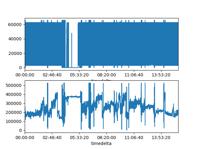
 print("Raw Signals: ")
 print(signals)

 # Plot
 fig, axes = plt.subplots(nrows=2, ncols=1)
 axes = axes.flatten()

 signals[0].plot(ax=axes[0])
 signals[1].plot(ax=axes[1])

 #==================
 #Bandpass Filtering
 #==================


 def bpf(signal):
     hp_filt_params = (1, 1) #(Hz, order)
     lp_filt_params = (20, 4) #(Hz, order)
     sampling_rate = 100
     filter = BandpassFilter(band_type='butter', fs=sampling_rate)
     filtered_signal = filter.signal_highpass_filter(signal, cutoff=hp_filt_params[0], order=hp_filt_params[1])
     filtered_signal = filter.signal_lowpass_filter(filtered_signal, cutoff=lp_filt_params[0], order=lp_filt_params[1])
     return filtered_signal

 signals['Filtered_Pleth'] = bpf(signals[0])
 signals['Filtered_IR_ADC'] = bpf(signals[1])

Out:

Raw Signals:
                          index      0       1
timedelta
0 days 00:00:00               0  36033  216524
0 days 00:00:00.010000        1  40919  216470
0 days 00:00:00.020000        2  45715  216415
0 days 00:00:00.030000        3  50227  216364
0 days 00:00:00.040000        4  54362  216379
...                         ...    ...     ...
0 days 15:37:43.720000  5626372  31408  183755
0 days 15:37:43.730000  5626373  31318  184002
0 days 15:37:43.740000  5626374  31117  184296
0 days 15:37:43.750000  5626375  30761  184554
0 days 15:37:43.760000  5626376  30261  184828

[5626377 rows x 3 columns]

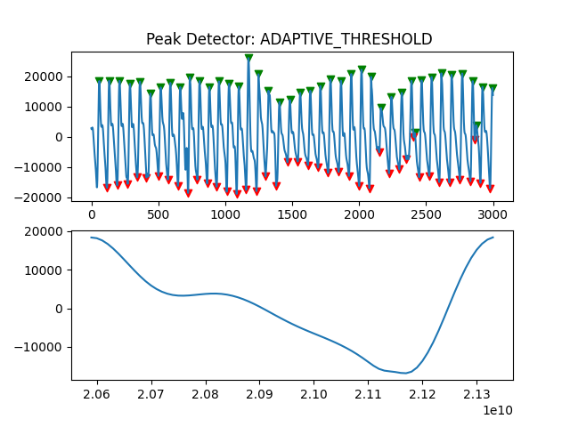
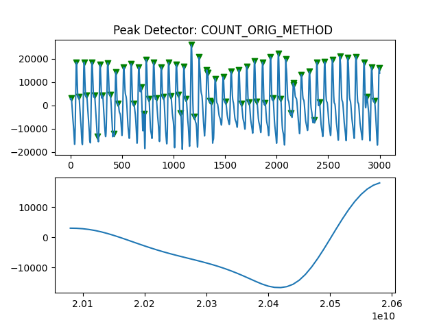
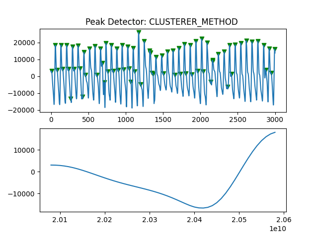
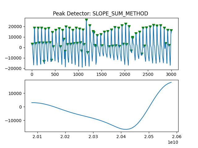
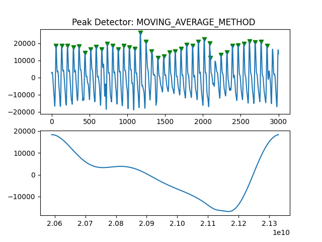
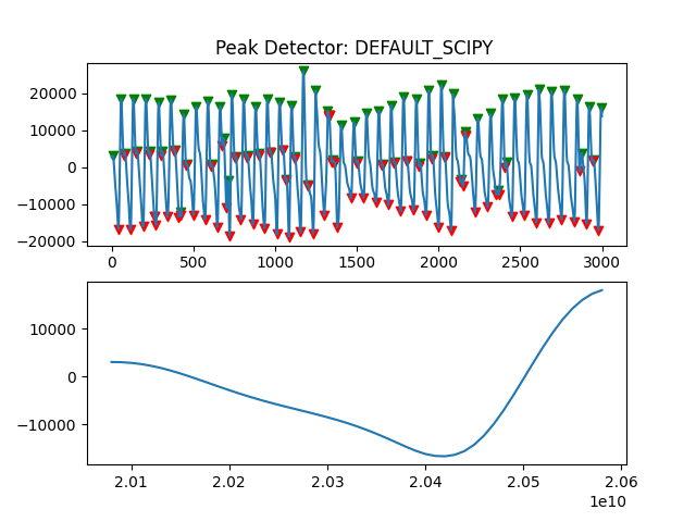
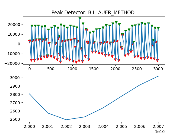
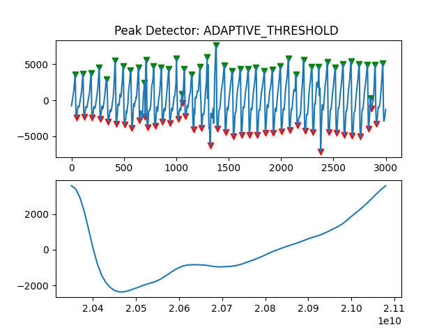
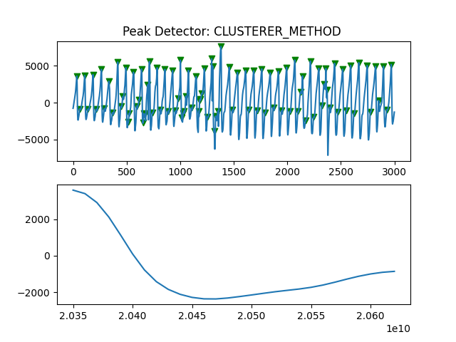
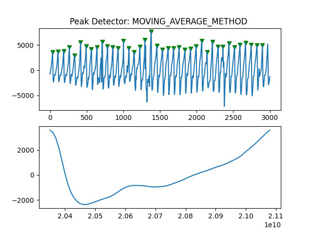
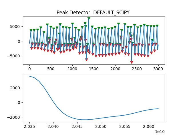
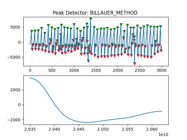
Peak Detector Comparison on PLETH

 print('Peak Detector Comparison on Pleth')
 pleth_segment= signals['Filtered_Pleth'][2000:5000]
 for i in range(1,8,1):
     peaks, troughs = PeakDetector().ppg_detector(pleth_segment, i)

     sample_range = np.arange(0,3000,1)
     fig, axes = plt.subplots(nrows=2, ncols=1)
     axes = axes.flatten()
     ax = axes[0]
     ax.plot(sample_range, pleth_segment)
     ax.scatter(peaks,pleth_segment[peaks], color="g", marker="v")
     ax.scatter(troughs,pleth_segment[troughs], color="r", marker="v")
     ax.title.set_text("Peak Detector: %s " %PeakDetectorNames[i-1])

     ax = axes[1]
     ax.plot(pleth_segment[peaks[0]:peaks[1]]) #plotting only one period

 plt.show

• 
• 
• 
• 
• 
• 
• 

Out:

Peak Detector Comparison on Pleth
the 'mode' parameter is not supported in the pandas implementation of take()
the 'mode' parameter is not supported in the pandas implementation of take()
search_for_onset() takes 3 positional arguments but 4 were given

<function show at 0x000001F0FFC0BD30>

Peak Detector Comparison on IR_ADC

 print("Peak Detector Comparison on IR_ADC")

 IRADC_segment= signals['Filtered_IR_ADC'][2000:5000]
 for i in range(1,8,1):
     peaks, troughs = PeakDetector().ppg_detector(IRADC_segment, i)

     sample_range = np.arange(0,3000,1)
     fig, axes = plt.subplots(nrows=2, ncols=1)
     axes = axes.flatten()
     ax = axes[0]
     ax.plot(sample_range, IRADC_segment)
     ax.scatter(peaks,IRADC_segment[peaks], color="g", marker="v")
     ax.scatter(troughs,IRADC_segment[troughs], color="r", marker="v")
     ax.title.set_text("Peak Detector: %s " %PeakDetectorNames[i-1])

     ax = axes[1]
     ax.plot(IRADC_segment[peaks[0]:peaks[1]]) #plotting only one period

 plt.show

• 
• 
• 
• 
• 
• 
• 

Out:

Peak Detector Comparison on IR_ADC
the 'mode' parameter is not supported in the pandas implementation of take()
the 'mode' parameter is not supported in the pandas implementation of take()
search_for_onset() takes 3 positional arguments but 4 were given

<function show at 0x000001F0FFC0BD30>

 '''

 Detector 6 and 7 seem to be performing better overall

 Note that the diacrotic notch can be higher than the diastolic peak
 and therefore, cannot be effectively detected by the peak detector.
 '''

Out:

'\n\nDetector 6 and 7 seem to be performing better overall\n\nNote that the diacrotic notch can be higher than the diastolic peak\nand therefore, cannot be effectively detected by the peak detector.\n'